
This post reviews three related developments in AI Planning, considering their impact on the AI field. In this context, planning refers to identifying a feasible sequence of actions and intermediate states that achieve a goal(s).
AI Planning methods can construct plans that can be evaluated for their efficiency (especially path length and time-to-generate), and can potentially be revised in execution.
I have chosen three historical milestones that are relevant to logistical planning (e.g. for air cargo):
- STRIPS (STanford Research Institute Problem Solver) [Fikes and Nilsson, 1971]
- Graphplan [Blum and Furst, 1997]
- HSP (Heuristic Search Planner) [Bonet and Geffner, 1999]
These are all classical planning approaches— best suited to a single agent in a fully observable, deterministic, and static environment. Such approaches usually aim to be domain-independent while being able to handle large problem spaces (with an exponential growth in the number of states relative to the size of the problem space). Classical planning is better suited to such complex, large problem spaces than alternatives such as regular search or logical inference (although it usually incorporates elements of these).
STRIPS
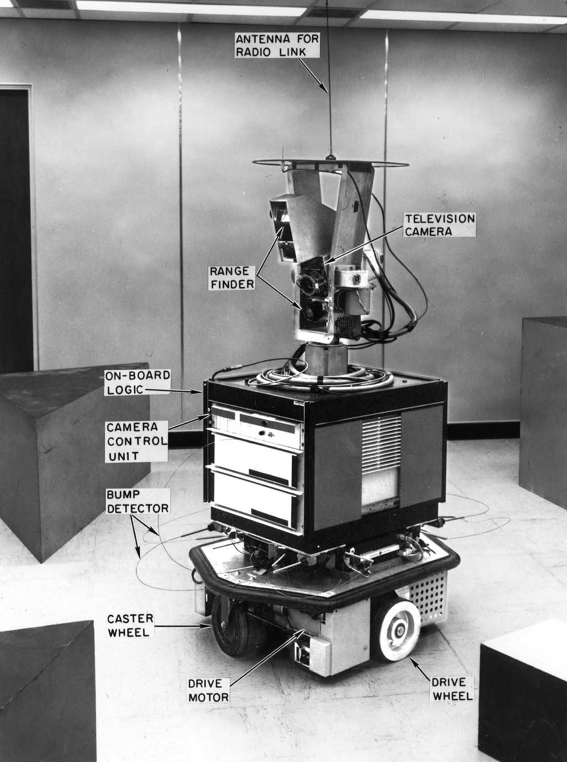
STRIPS (STanford Research Institute Problem Solver) was the planning module within the control system of Shakey, a robot developed at the Stanford Research Institute in the early 1970s [Fikes and Nilsson, 1971]. STRIPS was used to plan and direct Shakey’s actions to meet experimental goals in a world consisting of four rooms, where Shakey would be tasked with goals such as turning lights on and off or arranging boxes.
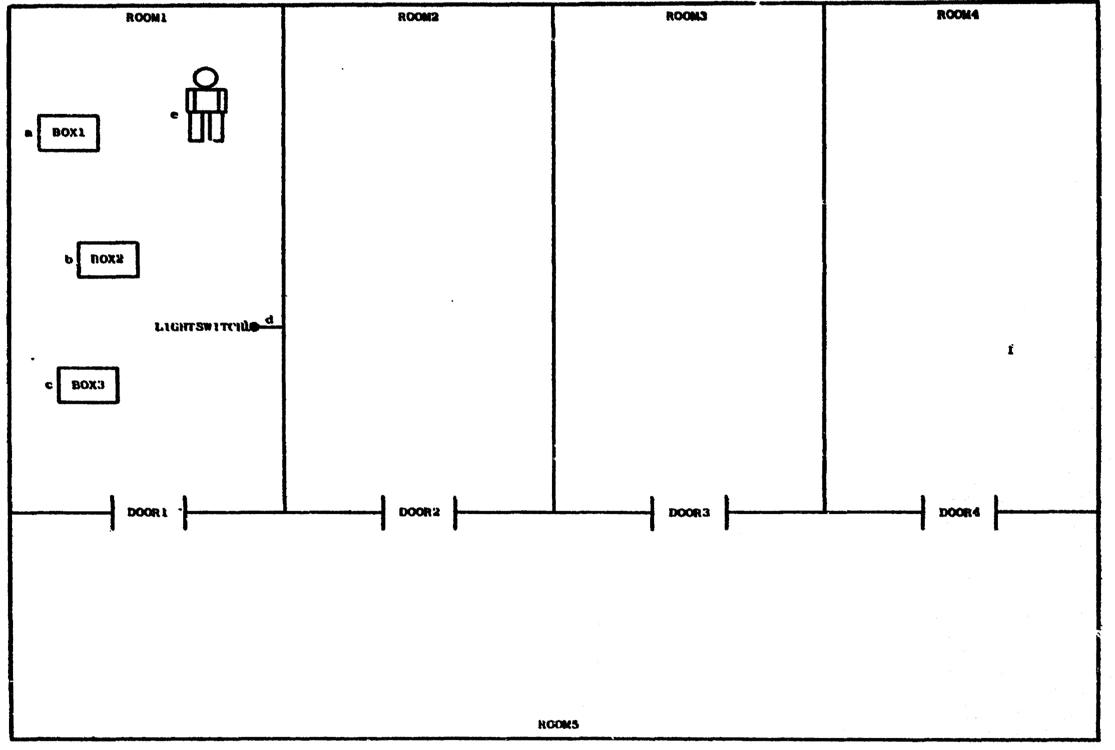 Figure 1: Shakey’s World
STRIPS is acknowledged as the first major AI planning solution (e.g. by [Russell and Norvig, 2010]), proving much more effective than its predecessors— most notably the GPS (General Problem Solver) [Newell and Simon, 1961]. However the most important contribution made by STRIPS was not its planning algorithms but instead its representation language, which is the focus of this discussion.
STRIPS’ representation language (hereafter called STRIPS for brevity) consisted of a first-order predicate schema and syntax for describing goals, objects, actions, effects, states (initial and intermediate), and rules/conditions (especially preconditions and postconditions). STRIPS could then be used to develop a sequential set of actions (plan) that could direct an actor to satisfy the goals given the initial world state and the constraints specified. An example of an initial state expressed in STRIPS is given below.
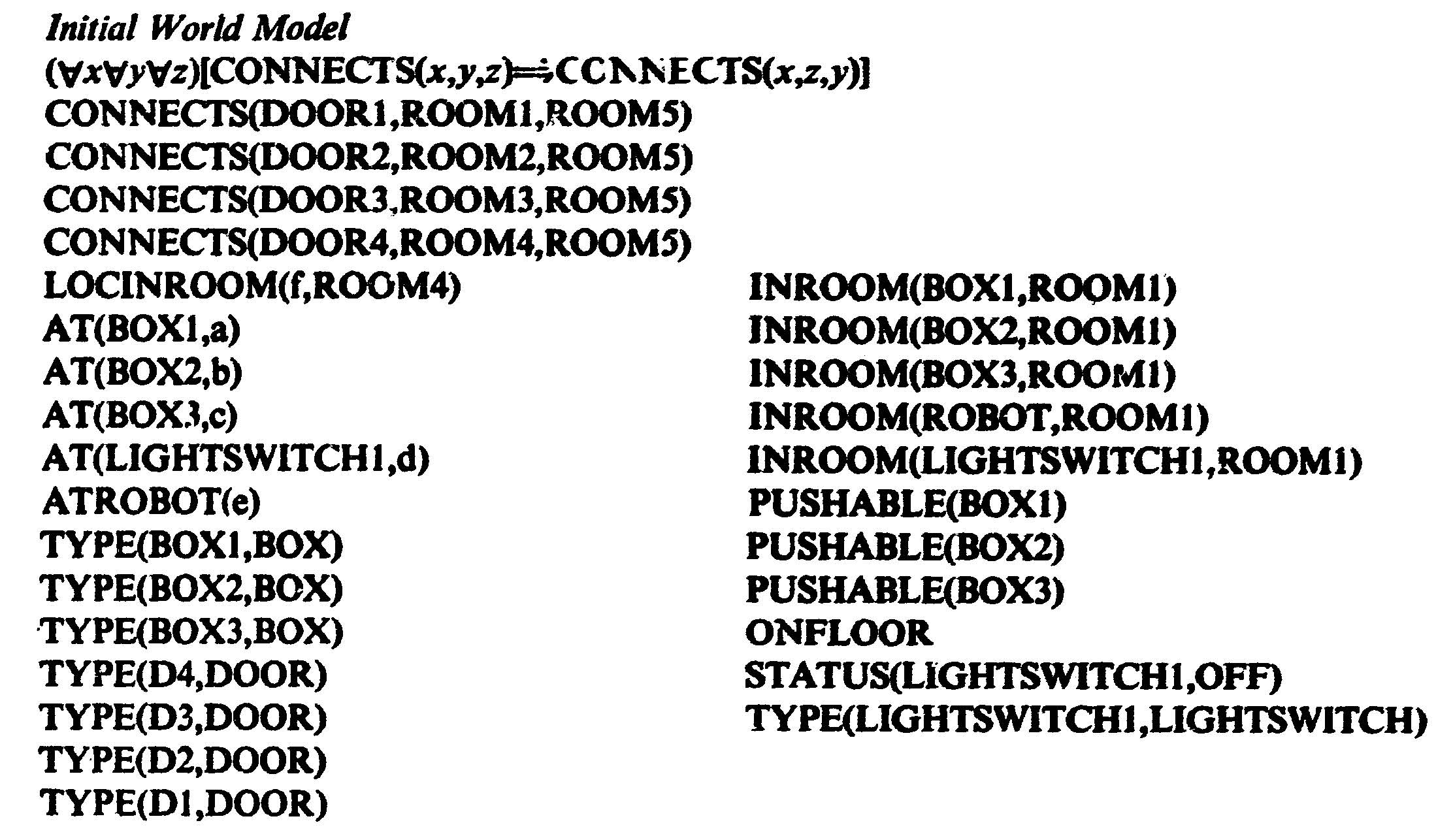
Figure 2: STRIPS Initial World State
STRIPS was unique at the time in that it:
- separates the description of the problem space from the approach used to find a plan, allowing the approach to be used with a variety of plan search methods;
- unlike more algebraic forms gives an effective and digestible representation of facts about the world state, possible actions, etc;
- gives a proposition that can be solved in polynomial time and space (if a solution exists) [Bylander, 1994];
- as evidenced by the success of the Shakey experiments (which themselves had a significant impact, including in fields such as cognition) helped make a significant leap in capability to solve complicated real-world problems; not merely the ‘toy problems’ in mostly abstract/virtual worlds that its predecessors were limited to.
STRIPS spawned descendent languages such as ADL [Pednault, 1986] and most notably PDDL [Ghallab et al, 1998], which has been incrementally developed to become a de-facto standard for describing planning problems.
Graphplan
Graphplan [Blum and Furst, 1997] revitalised planning with a propositional, graph-based approach instead of the partial-order planner method that had been predominant (as used by POP, SNLP, and others).
Graphplan was orders of magnitude faster than its predecessors, renewing interest in planning and a rapid development of other graph-based approaches. Graphplan allowed a simpler (but often more verbose) representation of a state space than POP et al, avoiding the need for variables in the planning process itself.
Graphplan can be used for problems expressed in a STRIPS-like representation, where it builds a plan graph in a first phase, and then performs a regression search in a second phase. The graph (of successive states and actions to reach a goal state) can be constructed in a manner that embeds useful information for constraining a later search into the graph itself. The graph is effectively a superset of valid plans, albeit missing the constraint that actions at a given time step do not interfere (allowing the graph to provide a constrained space that can be generated quickly).
Unlike the state space graphs that had been used prior, Graphplan’s planning graph was composed of:
- alternating levels of state nodes (fluents) and action nodes (with the first state level providing the initial state);
- ‘no-op’ actions to capture persistence of a fluent between state levels;
- edges connecting a state to actions for which it is a precondition; and,
- edges connecting actions to states that the action makes true or false (causes or prevents).
An example plan is shown below.
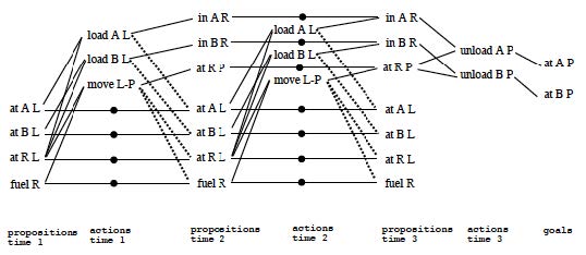 Figure 3: A Graphplan
Graphplan’s graph construction algorithm is guaranteed to include the optimal solution (it also has a termination guarantee when a solution cannot be found).
The main contributors to Graphplan’s efficiency are:
-
The encoding of an admissible relaxed heuristic into the graph for goal cost estimation, along with mutual-exclusivity rules for states and actions (mutexes). This allows a heuristic search (such as A* with iterative deepening) to efficiently find a successful plan.
-
Support for the generation and searching of valid parallel plans (as opposed to strict sequential ordering).
-
Memoization, i.e. updating the heuristic function from an unsuccessful iterative deepening search from a given node.
Graphplan inspired a number of other graph-based planners such as STAN [Fox and Long, 1998] and BlackBox [Kautz and Selman, 1998] — many of which are faster still than Graphplan.
Heuristic Search Planner (HSP)
The Heuristic Search Planner (HSP) was developed by Bonet and Geffner [1999] to utilise state-space search for large planning problems, with several variants being developed including HSP2 and HSPR.
Where Graphplan had trumped previous total order state-space planners, HSP led a resurgence in the approach by using a simple heuristic search cost estimate that is recomputed with each state level. This was competitive with other Graphplan-based planners at the time, as seen in the inaugural AIPS Planning Contest in 1998. HSP led to later descendants such as FF [Hoffman, 2001], which won the AIPS Planning Contest.
Like Graphplan, HSP uses a declarative STRIPS representation of the problem space and is also not domain-specific. Unlike Graphplan, HSP extracts a goal-reachability heuristic from this representation for a relaxed version of the problem (e.g. ignoring deletions), and instead of encoding this in a graph uses it to generate a cost estimate at each level to guide a heuristic search (e.g. BFS or A*). An estimate is used because determining the actual optimal cost is NP-hard.
Several variants of HSP were developed: HSP (a hill-climbing search planner); HSP2 (a best-first search planner); and HSPr (a regression search planner that searched backward from the goal using best-first search instead of forward from the initial state).
A number of search algorithms were used in earlier iterations of these (e.g. WA* for HSPr). HSPr also used a two-phase approach that is reminiscent of Graphplan— first propagating forward to estimate costs, and secondly searching backward for plans. However HSP2 with BFS gave best performance.
Subsequent methods have even combined Graphplan and HSP, such as AltAlt, which combined STAN (a Graphplan implementation) with HSPr [Srivastava et al 2001].
Conclusions
The three developments discussed above were significant and related milestones in the history of AI Planning.
STRIPS introduced a declarative construct for describing planning problems, with its descendants such as PDDL still being current.
Graphplan used STRIPS-based problem representation and introduced an encoded graph as an alternative to state space graphs that preceded it, with much better support for heuristic search alorithms such as A*.
Lastly, HSP (also STRIPS-based) did not use a planning graph but instead automatically derived a cost estimation heuristic from the problem definitions and dynamically calculated this at each level.
Many subsequent planners use elements of all three (e.g. AltAlt).
References
- Fikes, R. and Nilsson, N. (1971): STRIPS: A New Approach to the Application of Theorem Proving to Problem Solving
- Blum, A. and Furst, M. (1997): Fast Planning Through Planning Graph Analysis. Artificial Intelligence, 90 p:281–300.
- Bonet, B, and Geffner, H. (1999): HSP: Planning as Heuristic Search.
- Russel, S. and Norvig, P. (2010): Artificial Intelligence: A Modern Approach, 3rd Edition
- Bylander, T. (1994): The Computational Complexity of Propositional STRIPS Planning. Artificial Intelligence, 69 p:165-204.
- Srivastava, B. et al (2001): ALTALT: Combining Graphplan and Heuristic State Search. AI Magazine, vol 22, no. 3, pp. 88-90.